Geodata and base maps • BFS

library(BFS)
library(dplyr)
library(ggplot2)
library(sf) # install.packages("sf")

Base maps

bfs_get_base_maps() gives you the cartographic base maps of the BFS (the ThemaKart project) as sf objects. The first time, it downloads a zip file with several hundred files and saves it on your disk (a cache). bfs_clear_cache() deletes the cache.

switzerland <- bfs_get_base_maps(geom = "suis")
cantons <- bfs_get_base_maps(geom = "kant")
districts <- bfs_get_base_maps(geom = "bezk")
communes <- bfs_get_base_maps(geom = "polg")
capitals <- bfs_get_base_maps(geom = "stkt", type = "Pnts", category = "kk")
lakes <- bfs_get_base_maps(geom = "seen", category = "11")
rivers <- bfs_get_base_maps(geom = "flus", category = "22", type = "") # rivers have no type

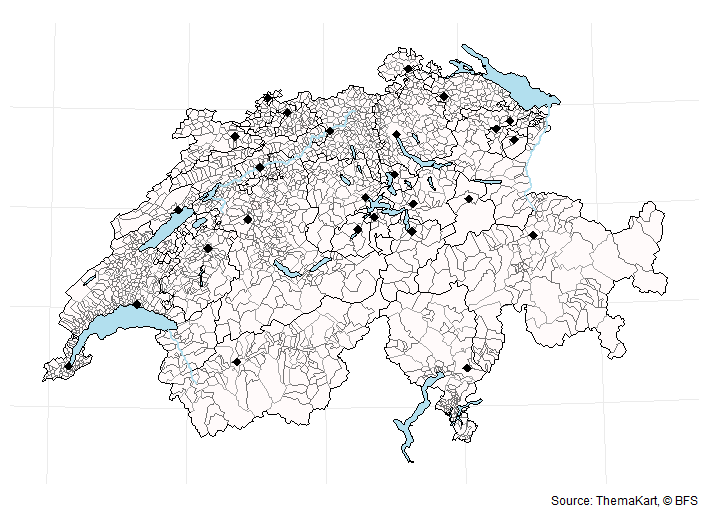
ggplot() +
  geom_sf(data = communes, fill = "snow", color = "grey45") +
  geom_sf(data = lakes, fill = "lightblue2", color = "black") +
  geom_sf(data = districts, fill = "transparent", color = "grey65") +
  geom_sf(data = cantons, fill = "transparent", color = "black") +
  geom_sf(data = rivers, color = "lightblue2", linewidth = 1) +
  geom_sf(data = capitals, shape = 18, size = 3) +
  theme_void() +
  labs(caption = "Source: ThemaKart, © BFS")

Map of Switzerland with its communes, districts, cantons, lakes, rivers and cantonal capitals

Choose a file

The name of each file is made of the arguments of bfs_get_base_maps(). For example, K4kant20220101gf_ch2007Poly.shp has the geometry kant, the date 20220101, the category gf (total area), the type Poly and the format shp.

Structure of a ThemaKart file name

By default, you get the most recent file. Use date for another date, for example date = "20230101". With return_sf = FALSE, you get the path of the file instead of an sf object. An argument set to "" matches all the values. For example, to list all the river files:

bfs_get_base_maps(geom = "flus", category = "", type = "", date = "", return_sf = FALSE)

By default, asset_number is the 2024 edition of ThemaKart. For another edition, give its asset number, for example "11927607" for 2020.

Interactive maps

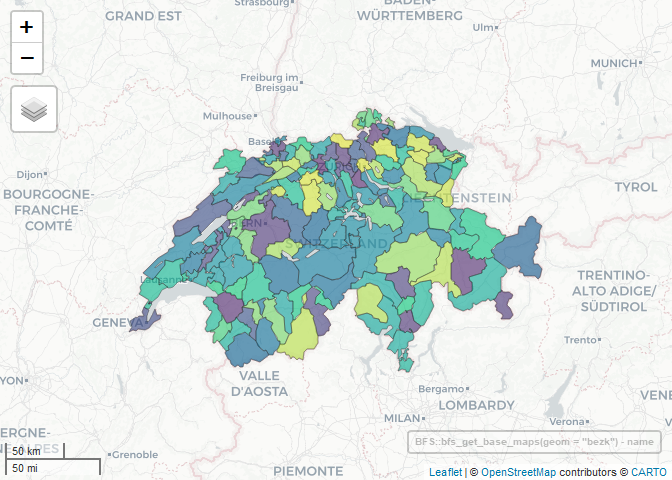
library(mapview)

bfs_get_base_maps(geom = "bezk") |>
  mapview(zcol = "name", legend = FALSE)

Interactive map of the Swiss districts

Join statistics

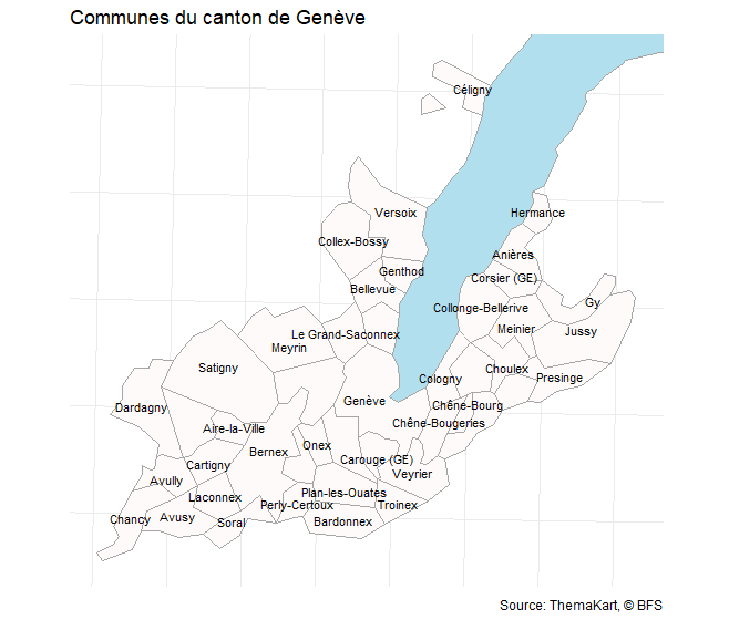
Each commune has its BFS number in the id column. You can join it with the list of communes in the package (register_gde), or with any BFS dataset by commune. For example, the communes of the canton of Geneva:

communes_ge <- bfs_get_base_maps(geom = "polg", date = "20230101") |>
  inner_join(filter(register_gde, GDEKT == "GE"), by = c("id" = "GDENR"))

lake_leman <- bfs_get_base_maps(geom = "seen", category = "11") |>
  filter(name == "Lac Léman")

bbox_ge <- st_bbox(communes_ge)

ggplot(communes_ge) +
  geom_sf(data = lake_leman, fill = "lightblue2", color = "grey65") +
  geom_sf(fill = "snow", color = "grey65") +
  geom_sf_text(aes(label = name), size = 3, check_overlap = TRUE) +
  coord_sf(xlim = bbox_ge[c("xmin", "xmax")], ylim = bbox_ge[c("ymin", "ymax")]) +
  theme_void() +
  labs(title = "Communes du canton de Genève", caption = "Source: ThemaKart, © BFS")

Map of the communes of the canton of Geneva

For the communes at another date, or for their history (mergers, new names), see the swissMunicipalities package.

Geodata of the Swiss geo-portal

The Swiss geo-portal publishes the geodata of the BFS and of other federal offices in a STAC API. bfs_get_catalog_geodata() lists its collections. It sends one request for each collection, so it takes a few minutes. Save the result:

catalog_geodata <- bfs_get_catalog_geodata()

catalog_geodata |>
  filter(grepl("^ch.bfs", collection_id)) |>
  select(collection_id, title)

Download the files of a collection with bfs_download_geodata() (you need the rstac package). The zip files are not extracted:

files <- bfs_download_geodata(
  collection_id = "ch.bfs.generalisierte-grenzen_agglomerationen_g1",
  output_dir = "borders_g1"
)
files

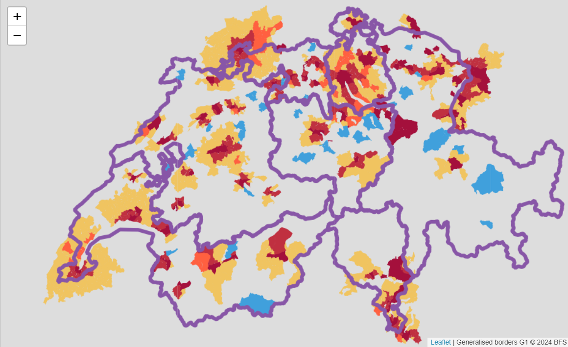
Some layers are also available as a Web Map Service (WMS). For example, with leaflet:

library(leaflet)

leaflet() |>
  setView(lng = 8, lat = 46.8, zoom = 8) |>
  addWMSTiles(
    baseUrl = "https://wms.geo.admin.ch/?",
    layers = "ch.bfs.generalisierte-grenzen_agglomerationen_g2",
    options = WMSTileOptions(format = "image/png", transparent = TRUE),
    attribution = "Generalised borders G2 © BFS"
  )

Leaflet map with the generalised borders of the BFS

You can use the geodata for free, but you must follow the terms of use of the Swiss geo-portal.