How to Create Interactive Maps with R
Use Case: Swiss maps
2024-03-25
What’s the plan for today?
- Access official geographic databases
- Join your own data to geographic datasets
- Create customized interactive maps (of Switzerland1)
Get all the R code of this talk: felixluginbuhl.com/talks
About me
- Currently supporting the R tranformation of the Statistical Office of St.Gallen.
- Worked 2 years as Data Scientist at the Global Fund.
- Background in social sciences (Master in Sociology and Master in European Studies from the University of Geneva).
Disclamer: I am a self-trained R mapper!1
Online presence: felixluginbuhl.com, github.com/lgnbhl.
How to access geodata?
International level:
- The Natural Earth Project (public domain).
European level:
- Gisco: Eurostat Mapping API.
Country level (Switzerland):
- Swiss national geoportal (geo.admin.ch)
- Official Thematic Base Maps (ThemaKart)
International geodata
Get world data from the Natural Earth Project.
```r .smaller #| echo: true #install.packages(“rnaturalearth”) library(rnaturalearth) library(ggplot2) library(sf)
world <- ne_countries(returnclass = “sf”)
ggplot(world) + geom_sf() + theme_minimal()
## International geodata

You also can access physical geodata with `ne_download()`.

```r
#| echo: true
rivers50 <- ne_download(
  scale = 50,
  type = "rivers_lake_centerlines",
  category = "physical",
  returnclass = "sf")

ggplot(rivers50) +
  geom_sf() +
  theme_minimal()
International geodata
Get national data with “country” argument (“geounit” for metropolitan only):
International geodata
Get “state” (cantonal) level data with ne_states().
European geodata
Access Eurostat Mapping API.
Switzerland geodata
Swiss national geoportal (Swiss Stac API) with bfs_get_catalog_geodata().
Switzerland geodata
The ThemaKart project gives access to various thematic maps.
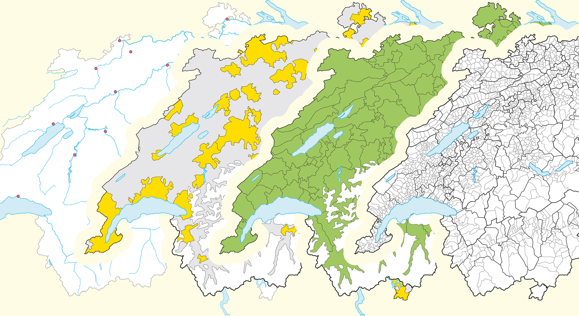
A typical base maps ThemaKart file looks like this:
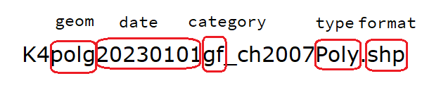
Switzerland geodata
You can access base maps files with bfs_get_base_maps().
#| echo: true
# list of geometry names: https://www.bfs.admin.ch/asset/en/24025645
switzerland_sf <- bfs_get_base_maps(geom = "suis")
communes_sf <- bfs_get_base_maps(geom = "polg", date = "20230101")
districts_sf <- bfs_get_base_maps(geom = "bezk")
cantons_sf <- bfs_get_base_maps(geom = "kant")
cantons_capitals_sf <- bfs_get_base_maps(geom = "stkt", type = "Pnts", category = "kk")
lakes_sf <- bfs_get_base_maps(geom = "seen", category = "11")
Switzerland static map with ggplot2
#| echo: true
library(ggplot2)

ggplot() +
  geom_sf(data = communes_sf, fill = "snow", color = "grey45") +
  geom_sf(data = lakes_sf, fill = "lightblue2", color = "black") +
  geom_sf(data = districts_sf, fill = "transparent", color = "grey65") +
  geom_sf(data = cantons_sf, fill = "transparent", color = "black") +
  geom_sf(data = cantons_capitals_sf, shape = 18, size = 3) +
  theme_minimal() +
  theme(axis.text = element_blank()) +
  labs(caption = "Source: ThemaKart, © BFS")
Joining data to Swiss geodata
Each observation of your data should be joined to a geodata spatial geometry.
The sf R package (for “Simple Feature”) allows to do it in a tidy way.
Joining data to Swiss geodata
Let’s download an official Swiss dataset with BFS:
r, results = 'hide' #| echo: true #bfs_get_catalog_data() # get catalog # Swiss dataset: https://www.bfs.admin.ch/asset/de/px-x-1502000000_101 swiss_students <- BFS::bfs_get_data( number_bfs = "px-x-1502000000_101", language = "fr", clean_names = TRUE)
Joining data to Swiss geodata
We can then pivot it and calculate share of female students:
#| echo: true
library(tidyverse)

swiss_students_gender <- swiss_students |>
  filter(nationalite_categorie == "Suisse", #only Swiss students
         canton_de_lecole != "Suisse") |> #only cantonal data
  pivot_wider(names_from = sexe, values_from = eleves_et_etudiants) |>
  mutate(share_woman = round(Femme/`Sexe - Total`*100, 1))

glimpse(swiss_students_gender)
Joining data to Swiss geodata
We can then joining our data to the geodata.
Joining data to Swiss geodata
We need to do some recoding before the left join.
#| echo: true
swiss_student_map <- swiss_students_gender %>%
  filter(canton_de_lecole != "Schweiz") %>% # remove national level
  mutate(canton_de_lecole = str_remove(canton_de_lecole, ".*/"),
         canton_de_lecole = str_trim(canton_de_lecole),
         canton_de_lecole = recode(canton_de_lecole, "Berne" = "Bern", "Freiburg" = "Fribourg", "Grischun" = "Graubünden", "Ticino" = "Tessin", "Wallis" = "Valais")) |>
  left_join(swiss_map, by = c("canton_de_lecole" = "name")) |>
  select(canton_de_lecole, annee, degre_de_formation, share_woman, geometry)

glimpse(swiss_student_map)
Joining data to Swiss geodata
To ease your work with geodata names, I provided the Swiss official registers.
Interactive Maps with mapview
mapview provides functions to very quickly and conveniently create interactive visualisations of spatial data. It’s main goal is to fill the gap of quick (not presentation grade) interactive plotting to examine and visually investigate both aspects of spatial data, the geometries and their attributes. It can also be considered a data-driven API for the leaflet package as it will automatically render correct map types, depending on the type of the data (points, lines, polygons, raster).
Source: https://r-spatial.github.io/mapview/
Interactive Maps with mapview
The easy way with mapview (but limited customization).
Interactive Maps with mapview
Using mapview with our Swiss students dataset.
#| echo: true
swiss_student_map_pivoted <- swiss_student_map |>
  pivot_wider(names_from = "degre_de_formation", values_from = "share_woman") |>
  sf::st_as_sf()

swiss_student_map_pivoted |>
  filter(annee == "2022/23") |>
  mapview(zcol = "Degré de formation - Total", layer.name = "% étudiantes suisses, 2023")
Interactive Maps with mapview
mapview is using Leaflet in the background, which allows to access extra functionality:
#| echo: true
map_2023 <- swiss_student_map_pivoted |>
  filter(annee == "2022/23") |>
  mapview(zcol = "Degré de formation - Total", layer.name = "% étudiantes suisses, 2023")

map_2000 <- swiss_student_map_pivoted |>
  filter(annee == "1999/00") |>
  mapview(zcol = "Degré de formation - Total", layer.name = "% étudiantes suisses, 2000")
Interactive Maps with mapview
mapview is using Leaflet in the background, which allows to access extra functionality:
Interactive Maps with mapview
mapview is using Leaflet in the background, which allows to access extra functionality:
Interactive Maps with mapview
mapview is using Leaflet in the background, which allows to access extra functionality:
Interactive Maps with leaflet
Let’s reproduce this datawrapper map:
Interactive Maps with leaflet
Let’s find the data with bfs_get_catalog_tables().
Interactive Maps with leaflet
Let’s download and read the data.
Interactive Maps with leaflet
Let’s download and read the data.
Interactive Maps with leaflet
Top 5 by commune by rank and percent:
Interactive Maps with leaflet
Create html table for each commune
#| echo: true
create_table <- function(name) {
  df <- df_top_5 |>
    filter(GDENAME == name)

  table <- df |>
    select("Rank" = RANK, "Last name" = LASTNAME,
           "Number" = VALUE, "Percentage" = PCT_GDE) |>
    mutate(Rank = paste0(Rank, "."),
           Percentage = paste0(Percentage, "%")) |>
    kableExtra::kable(format = "html", align = "llrr")

  paste0(
    "<b>", unique(df$GDENAME), "</b><br>",
    table
  )
}
Interactive Maps with leaflet
Interactive Maps with leaflet
Add html table code in the table column.
Interactive Maps with leaflet
Get official Swiss base maps.
Interactive Maps with leaflet
Join our data with geodata.
Interactive Maps with leaflet
Create a basic leaflet map.
#| echo: true
library(leaflet)

# customize legend
bins = c(0, 1, 2.5, 5, 10, 20, 100)
col_custom = c("#f5b3bb", "#ef8894","#e85767","#dc0018","#a60013","#73000d")
pal <- colorBin(col_custom,
                domain = sf_communes_joined$PCT_GDE,
                bins = bins)
legend_labels <- c("0 – 1", "1 – 2.5", "2.5 – 5",
                   "5 – 10", "10 – 20", "20 – 100")

map <- leaflet(sf_communes_joined, height = 600, width = 900) |>
  addPolygons(
    weight = 0.3,
    opacity = 1,
    color = "white",
    fillOpacity = 1,
    fillColor = ~pal(PCT_GDE),
    label = ~lapply(table, htmltools::HTML),
  ) |>
  addPolygons(
    data = lakes_sf,
    label = ~name,
    stroke = FALSE,
    color = "gray70"
    ) |>
  addLegend(
    title = "Share of the most<br>common surname, in %",
    labFormat = function(type, cuts, p) { paste0(legend_labels) },
    values = ~PCT_GDE,
    pal = pal,
    opacity = 1
  )
Interactive Maps with leaflet
Create a basic leaflet map.
Interactive Maps with leaflet
Adding bounding box, empty background and fix zooming.
#| echo: true
# get bounding box of Switzerland
bbox <- st_bbox(sf_communes_joined) |>
  as.vector()

map_final <- map |>
  addTiles(urlTemplate = "", # empty background
           options = providerTileOptions(minZoom = 8, maxZoom = 12)) |>
  setMaxBounds(lng1 = bbox[1], lat1 = bbox[2],
               lng2 = bbox[3], lat2 = bbox[4]) |>
  leaflet.extras::setMapWidgetStyle(style = list(background = "transparent"))
Interactive Maps with leaflet
Adding bounding box, empty background and fix zooming.
Interactive Maps with leaflet
Add map in a card with title and legend.
#| echo: true
library(bslib)
library(htmltools)

card <- card(
  tags$h5("The Five Most Frequent Last Names by Commune, 2022"),
  tags$i("Hover to display the five most common surnames (actual number and percentage) by commune."),
  map,
  tags$p(
    "Source: FSO – STATPOP, inspired by:",
    tags$a("https://www.bfs.admin.ch/asset/en/27205601",
           href = "https://www.bfs.admin.ch/asset/en/27205601")),
  tags$p("Get the R code:",
         tags$a("felixanalytix.com",
                href = "https://felixanalytix.com")),
  min_height = 800,
  max_height = 800
)
Interactive Maps with leaflet
Add map in a card with title and legend.
Any questions?
Get the R code of this talk:
You can contact me on LinkedIn:
Thank you for your attention!